 From the Pigeon Lab to the Courtroom
John T. Wixted
University of California, San Diego
Reading Options:
Continue reading below, or:
Read/Download PDF | Add to Endnote
Abstract
The task of detecting the presence or absence of a stimulus based on a diagnostic evidence variable is a pervasive one. It arises in basic experimental circumstances, such as a pigeon making a decision about whether or not a stimulus was presented 10 seconds ago, as well as in applied circumstances, such as a witness making a decision about whether or not a suspect is the guilty perpetrator. Understanding how to properly conceptualize and analyze performance on a signal-detection task like that is nontrivial, and advances in this area have come mainly from experimental psychologists studying performance on basic memory and perception tasks. One illustrative example from the pigeon memory literature is considered here in some detail. Unfortunately, lessons learned by basic experimental psychologists (e.g., the value of using signal-detection theory to guide thinking, appreciating the distinction between discriminability and response bias, understanding the utility of receiver operating characteristic analysis, etc.), while having a major impact on applied fields such as diagnostic medicine, have not always been fully appreciated by applied psychologists working on issues pertaining to eyewitness misidentification. In this regard, signal-detection-based analyses can greatly enhance our understanding of important applied issues such as (a) the diagnostic accuracy of different police lineup procedures and (b) the relationship between eyewitness confidence and accuracy. The application of signal-detection theory to issues like these can reverse what many believe to be true about eyewitness identifications made from police lineups.
Keywords: Keywords: pigeon memory; ROC analysis; signal-detection theory; eyewitness memory, confidence and accuracy
Author Note: John T. Wixted, Department of Psychology, University of California, San Diego.
Correspondence concerning this article should be addressed to John T. Wixted at jwixted@ucsd.edu.
A ubiquitous task, both in the laboratory and in everyday life, involves making a decision about whether a stimulus occurred (Outcome A) or not (Outcome B). A pigeon, for example, might have to decide whether a keylight was briefly presented 5 s ago (Outcome A) or not (Outcome B) by pecking a red choice key (decision: the keylight was presented) or a green choice key (decision: the keylight was not presented). Similarly, a human might have to decide whether a test word appeared on a previously presented list (Outcome A) or not (Outcome B) by saying “old” or “new.” Or an eyewitness to a crime might have to decide whether a person shown to them by the police is the one who committed the crime (Outcome A) or not (Outcome B) by making a positive identification or not. These examples are all from the domain of memory, but similar detection tasks come up in many other domains. In diagnostic medicine, for example, a patient has an illness (Outcome A) or not (Outcome B) and a medical test is used to make a decision about which condition applies to this patient. And in a jury trial, the defendant is guilty (Outcome A) or not (Outcome B), and the jury makes a decision to convict or not. In all of these cases, a binary (dichotomous) decision has to be made based on what is often assumed to be a continuous evidence variable. The question facing the decision maker in each of these cases is whether or not there is sufficient evidence along some continuous scale to warrant making the decision to classify the item into Outcome A or not.
The continuous evidence variable upon which the decision is based changes as a function of the task, but the decision-making logic is the same in each case. On recognition memory tasks, the continuous evidence variable is, theoretically, the internal strength of the memory signal (which ranges from low to high), and the question is whether or not the memory signal is strong enough to say (for example) that the suspect in the photo is the person who committed the crime. In the medical context, the continuous variable might be the blood count of some protein, and the question is whether or not the blood count is high enough to warrant the diagnosis. And in a jury trial, the evidence variable is literally the sum total of incriminating evidence against a defendant. Is there enough evidence to conclude that the defendant is guilty beyond a reasonable doubt or not?
Signal-detection theory offers an illuminating framework for understanding how decisions like these are made (Green & Swets, 1966; Macmillan & Creelman, 2005). It not only provides a way to conceptualize why one decision is made instead of the other; it also suggests a measurement strategy that one would not likely hit upon in its absence. That measurement strategy is called receiver operating characteristic (ROC) analysis. ROC analysis has two broad purposes: (a) to distinguish between competing theories of decision making (e.g., between two nonidentical signal-detection models, or between a signal-detection model and a non-detection model), and (b) to measure discriminability (i.e., the ability to distinguish between the two relevant states of the world) in theory-free fashion. The second purpose may be the more important of the two because it is how ROC analysis is used in applied settings (such as diagnostic medicine). It might seem counterintuitive that a method like ROC analysis, which is so closely tied to signal-detection theory, can be described as “theory free,” but it is. Signal-detection theory brings you to and helps you conceptualize ROC analysis—indeed, it is hard to imagine conceiving of that approach in the absence of signal-detection theory—but once it does, for applied questions, the theory is no longer needed to interpret the data.
Using ROC Analysis to Test Theory
My own introduction to signal-detection theory (which eventually brought me to ROC analysis) began with a pigeon memory task. In a typical delayed matching-to-sample task, a trial begins with the presentation of (for example) a red or green light and then, after a delay, red and green choice keys are presented simultaneously. A response to the matching color is rewarded with food, whereas a response to the non-matching color ends the trial. A variant of this basic task involves the use of initial sample stimuli that are asymmetric in salience. For example, some investigations have involved sample stimuli consisting of presentations of food versus no food. Typically, the presentation of one of these samples is followed, after some delay, by a choice between two comparison stimuli (e.g., red and green). A response to one comparison is reinforced following samples of food, and a response to the other comparison is reinforced following samples of no food. A consistent finding in these studies is that performance following samples of food declines as the retention interval increases, whereas performance following samples of no food does not (Colwill, 1984; Colwill & Dickinson, 1980; Grant, 1991; Wilson & Boakes, 1985).
The same asymmetrical decay functions were observed by Grant (1991) when samples consisted of the presence versus absence of a variety of stimuli (including colors, shapes, and food). In each case, performance following the presence of an event declined as the retention interval increased, but performance following the absence of an event did not. In still other cases, the sample stimuli consisted of a short-duration houselight (e.g., 2 sec) versus a long-duration houselight (e.g., 10 sec), or a white keylight that required 40 keypecks to extinguish it versus a white keylight that required only 10 keypecks (Colwill, 1984; Fetterman & MacEwen, 1989; Sherburne & Zentall, 1993; Spetch & Wilkie, 1983). In these cases, too, the forgetting functions following the two samples are usually asymmetric. Figure 1 shows an example of asymmetric forgetting functions from a sample/no-sample task (Wixted, 1993).
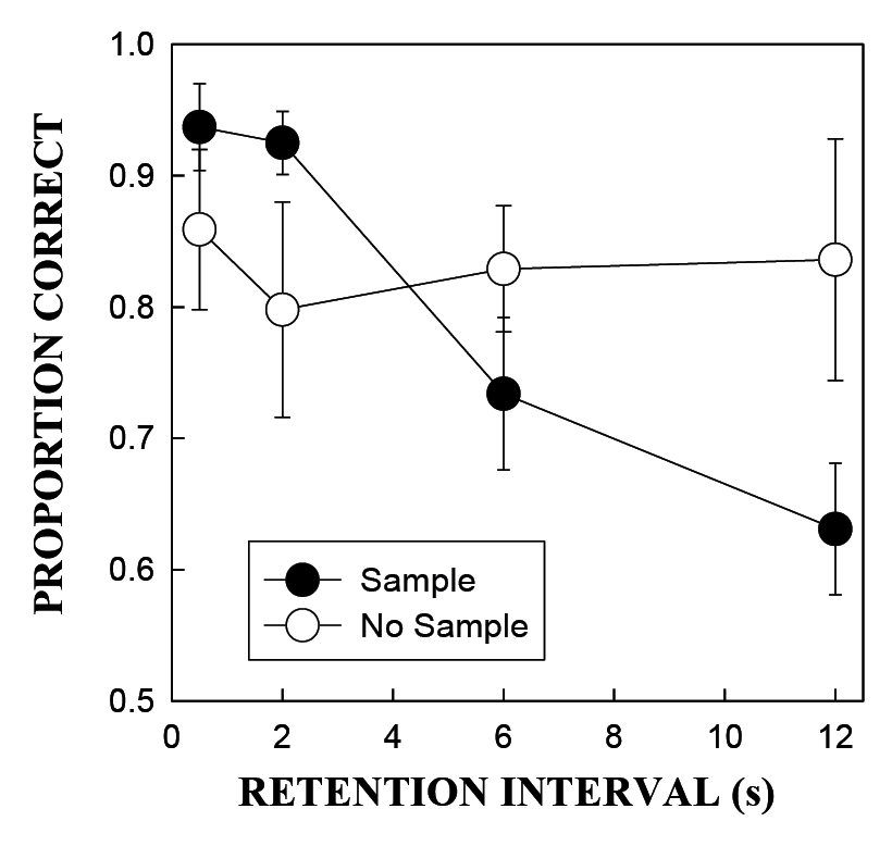
Figure 1. Average hit rate (proportion of correct responses on sample trials) and correct rejection rate (proportion of correct responses on no-sample trials) as a function of retention interval for pigeons in Experiment 1 of Wixted (1993). (The error bars represent the standard errors associated with each mean value.)
Typically in these experiments, performance following the less salient sample (e.g., no sample, no food, a short sample, or a sample requiring relatively few keypecks) begins at a high level and remains accurate as the delay interval increases. Performance following the more salient sample (e.g., a sample in a sample/no-sample procedure, food in a food/no-food procedure, a long sample, or a sample requiring many keypecks) decreases rapidly as the retention interval increases and eventually falls to well below 50% correct (if the retention interval is long enough). What explains that pattern? Below, I present two competing theoretical accounts in some detail and describe an empirical investigation designed to differentiate between them. The following discussion may seem far removed from important social questions such as how to minimize eyewitness misidentifications, but my contention is that any such impression is far from the truth.
The Default Response (High-Threshold) Hypothesis
Various theories have been offered to account for asymmetric forgetting functions, but one theory is of particular interest because of its close connection to a theory of human recognition memory that prevailed in the years prior to the introduction of signal-detection theory. Colwill (1984), Wilson and Boakes (1985), and Grant (1991) all argued that the absence of a retention interval effect on no-sample trials suggests that memory plays no role on these trials. Instead, in the absence of memory, pigeons theoretically adopt a default response strategy of choosing the comparison stimulus associated with the absence of a sample. The default strategy is overridden on trials involving a sample so long as the memory trace has not completely faded. This explanation accounts for the flat retention function on no-sample trials because, whether the retention interval is short or long, no memory trace is ever present to override the default response. The same account explains why performance on sample trials is often significantly below chance at longer retention intervals: When the memory trace fades completely, subjects revert to their default strategy and reliably choose the wrong comparison stimulus.1
A theory along these lines makes perfect sense, but one important and nonobvious feature of the theory is its implicit assumption that memory for the sample exists in one of only two discrete states, present vs. absent (i.e., memory strength is construed as an all-or-none variable, not as a continuous variable). According to this theory, when memory for the sample is present, that memory guides the response, leading to a correct choice. When memory for the sample is not present, the default response is implemented instead. If memory operated in that fashion, then a simple, algebraic model could be applied to the data to estimate a variable of interest, namely, the proportion of sample trials in which the sample was remembered (p). Imagine that, for a given task, the true value of p happened to be .80 (i.e., on 80% of the sample trials, the sample is remembered and guides choice performance). What might the pigeon do on the 20% of sample trials (and on 100% of the no-sample trials) in which memory for the sample is absent? The assumption is that on these trials, the pigeon implements its default strategy of choosing the no-sample alternative. The default strategy might not be to always choose the no-sample alternative under no-memory conditions, so the probability of choosing the no-sample alternative in the absence of memory can be represented by d, where d falls between 0 and 1. The value of d might be 1.0 (the pure default-response model), or it might instead be .90 or .80 without changing the basic pattern of results that this model predicts.
Generally speaking, the probability of choosing the sample alternative on a sample trial, p(“S” | S), is p (the probability that the sample is remembered) + (1 – p) times (1 – d), where 1 – p is the probability that the sample is not remembered and 1 – d is the probability that the sample alternative is selected on no-memory trials. If d = 1.0, then determining p is simple and straightforward: one need only measure the proportion of sample trials in which the sample alternative is chosen because p(“S” | S) = p + (1 – p) × (1 – d) = p + (1 – p) × 0 = p. Across conditions, one might find that the value of p is .80 in conditions involving a short retention interval and .20 in conditions involving a long retention interval (i.e., the probability of remembering the sample on sample trials decreases as the retention interval increases).
If the value of d is not equal to 1.0, then determining the value of p is slightly more complicated but still easy to do. The value of d is first determined by measuring the proportion of no-sample trials in which the no-sample alternative is correctly chosen. Imagine that on no-sample trials, pigeons choose the no-sample alternative 90% of the time (d = .90). This result would mean that when no memory for the sample is present (as must be true on no-sample trials), the bird’s default response is to choose the no-sample alterative 90% of the time and to choose the sample alternative 10% of the time. If d = .90, then performance on sample trials no longer provides a direct readout of p because, as indicated above, sample trial performance is theoretically equal to p + (1 – p) × (1 – d). Note that we can replace 1 – d with g, where g is the probability of “guessing” that the sample was presented despite no memory for the sample. Because g = 1 – d, we can write the equation as p(“S” | S) = p + (1 – p) × g.
If the observed probability of correctly choosing the sample alternative on sample trials, p(“S” | S), is called the hit rate (HR) and the observed probability of incorrectly choosing the sample alternative on no-sample trials, p(“S” | NS), is called the false alarm rate (FAR), then this simple model yields two equations:
HR = p + (1 – p) × g(1)
and
FAR = g(2)
This model is diagrammed in Figure 2. Note that the equation for performance on no-sample trials (Equation 2) places the focus on the non-default response (i.e., the probability of choosing the sample alternative by default in the absence of memory), but it is just another way of indicating that on no-sample trials, the probability of correctly choosing the no-sample alternative is equal to 1 – g, which is to say that it equals d.
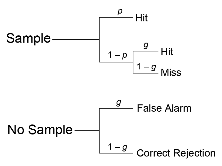
Figure 2. Illustration of the high-threshold account of recognition memory. On sample trials, with probability p, the sample is remembered and the sample choice alternative is chosen (a hit). With probability 1 − p, the sample is not remembered and the default response of choosing the no-sample choice alternative with probability d is implemented. Because d = 1 − g, this means that, with probability g, the sample choice alternative is chosen (a hit). With probability 1 − g, the no-sample choice alternative is chosen (a miss). On no-sample trials, memory is never present so the default response is always implemented. Thus, with probability g, the sample choice alternative is chosen (a false alarm). With probability 1 − g, the no-sample choice alternative is chosen (a correct rejection).
Whereas the false alarm rate on no-sample trials provides a direct estimate of g, the hit rate on sample trials must be corrected to estimate p. This can easily be done by substituting FAR from Equation 2 for g in Equation 1:
HR = p + (1 – p) × FAR(3)
With a little algebraic rearrangement, we can solve for p to yield:
p = (HR – FAR) ∕ (1 – FAR)(4)
Using this equation, actual memory-based performance on sample trials can be directly computed from the data.
A concrete example will show how these equations work. Imagine that the size of the retention interval is manipulated within session, and performance on sample trials is 80% correct on short retention interval trials (HRshort = .80) and 40% correct on long retention interval trials (HRlong = .40). Further imagine that on no-sample trials, the no-sample alternative is correctly chosen by default 80% of the time. In other words, for both short and long retention intervals, d = .80 and g = .20. Using the equations above, we can estimate p for short and long retention interval trials:
pshort = (.80 – .20) ∙ (1 – .20) = .60 ∙ .80 = .75
plong = (.40 – .20) ∙ (1 – .20) = .20 ∙ .80 = .25
In other words, when the retention interval is short, the bird remembers the sample on 75% of the trials, but when the retention interval is long, the bird remembers the sample on only 25% of the trials.
This algebraic approach to conceptualizing memory performance corresponds exactly to how recognition memory theorists once conceptualized human recognition memory performance on list-learning tasks. The theory was called the high-threshold theory of recognition memory (Green & Swets, 1966). In fact, although rarely used today, Equation 4 is the standard correction for guessing formula that was often used to measure recognition memory performance in list-learning experiments with humans (Macmillan & Creelman, 2005).
Perhaps the most important point to appreciate here is that, according to this model, various intuitively appealing measures of performance fully conflate two distinct properties of the decision-making process that ought to be separately estimated. For example, consider the most obvious choice of a dependent measure on a sample/no-sample task, overall proportion correct. Expressed in terms of the hit rate and false alarm rate, proportion correct is equal to [HR × NSample + (1 – FAR) × NNo-sample ] ∙ N, where NSample = the number of sample trials, NNo-sample = the number of no-sample trials, and N = NSample + NNo-sample (i.e., N = the total number of trials). If NSample = NNo-sample, as would typically be true, then proportion correct reduces to:
Proportion correct = [HR + (1 – FAR) ] ∙ 2(5)
Note that 1 – FAR is simply the proportion correct on no-sample trials, so this expression is the average of proportion correct on sample and no-sample trials.
Consider next what this proportion correct measure theoretically captures using the high-threshold model as a guide. We know from Equations 1 and 2 that HR = p + (1 – p) × g and FAR = g. Substituting these expressions for HR and FAR in Equation 5 yields:
Proportion correct = [p + (1 – p) g + (1 – g)] ∙ 2
which reduces to:
Proportion correct = [p (1 – g) + 1] ∙ 2
Thus, according to this model, if the ability to remember the sample remains constant across conditions but the likelihood of guessing changes across conditions, proportion correct will change. This change in the performance might lead the experimenter to conclude that memory in one condition is better than memory in the other, but that conclusion would be a mistake. The use of Equation 4 would reveal that memory is actually the same across both conditions (assuming that the high-threshold theory is correct).
From the perspective of high-threshold theory, p is the key measure. It is, for example, the measure that would be expected to be impaired in a group of amnesic patients (for humans tested using list memory), and it is the measure that would be expected to decrease as the retention interval increased (on a sample/no-sample task with birds or a list-memory task with humans). In addition, and critically, p would also be expected to remain constant (but the hit and false alarm rates would change) if the only aspect of performance that changed across conditions was g. According to Equations 1 and 2, both the hit rate and false alarm rate would be expected to increase as g increased, and both would decrease as g decreased. But only p is a measure of the ability to discriminate between the two states of the world. If p = 0, then performance on sample and no-sample trials would be the same (HR = FAR). In that case, the bird would show no evidence of being able to discriminate sample from no-sample trials. If p = 1, then performance on sample and no-sample trials would always be perfect if g = 0 (though it could be as low as 50% correct if g = 1).
The value of g is an experimentally manipulable variable. For example, a high rate of guessing (i.e., a high value of g) can be induced by arranging a differentially high payoff for correct sample choices (for pigeons) or correct “old” decisions (for humans on a list-learning task). A low rate of guessing (i.e., a low value of g) can be induced by arranging a differentially high payoff for correct no-sample choices (for pigeons) or correct “new” decisions (for humans on a list-learning task). This means that a set of hit and false alarm rate pairs, each of which is theoretically associated with a single level of memory-based performance (i.e., a single level of p), can be obtained across conditions by varying g. With those data in hand, one can plot hit rate vs. false alarm rate, and the resulting plot is known as the ROC.
Critically, Equation 3 provides the predicted shape of the ROC. That equation is in the form of the familiar equation for a straight line, y = m × x + b. In other words, according to Equation 3, the ROC, which is a plot of HR vs. FAR with memory (p) held constant, should be linear. The problem is that empirical ROCs are almost invariably curvilinear, which is why this simple model has been rejected, both in studies of human memory and (sometimes) pigeon memory. Signal-detection theory, which is considered next, offers a more viable interpretation of ROC data. For the moment, the most important take-home message is that a theoretical analysis of performance on a detection task draws a distinction between two distinct aspects of memory performance: response bias vs. the ability to differentiate between the two relevant states of the world. It is easy to lose sight of the importance of this distinction, which is what happened when researchers investigated recognition memory in the real world (an issue addressed later in this article).
Signal-Detection Theory
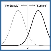
Figure 3 illustrates the signal-detection interpretation of performance on the sample/no-sample task (Wixted, 1993). The x-axis in this case represents the subjective strength of memory that a sample was presented earlier in the trial. Whereas the threshold model assumes the complete absence of a memory signal on these trials (which is intuitively sensible given that no sample was presented), the signal-detection model instead assumes that the act of retrospection always produces at least some false sense of sample occurrence. This is its most theoretically interesting departure from the high-threshold model. The strength of that false memory signal will vary from trial to trial due to noise in the neural system, but its mean value will be relatively low. Everything is the same on sample trials except that the average strength of the memory signal will be higher. Because the two distributions of memory strength signals partially overlap, there is no specific memory strength value that perfectly distinguishes between sample trials and no-sample trials. This is why the theory assumes that a criterion memory strength value, c, is set. On any trial in which the memory strength value exceeds the criterion, the sample alternative is chosen. This includes some no-sample trials in which the memory strength signal happens to be arbitrarily high. Thus, a false alarm in this model is based on a strong enough false memory signal, not on a random guess that occurs despite the complete absence of a memory signal (as in the threshold model). The proportion of the no-sample distribution that exceeds the criterion represents the false alarm rate. The proportion of the sample distribution that exceeds the criterion represents the hit rate. In this example, the hit rate ≈ .93 and the false alarm rate ≈ .07.

Figure 3. A graphical illustration of signal-detection theory. According to this theory, the memory system always has some subjective sense that the sample was presented, and the strength of that signal varies from trial to trial. On no-sample trials, the mean of the distribution is low, whereas on sample trials it is higher. On a given trial, the sample choice alternative is chosen if the strength of the memory signal exceeds the decision criterion, c. Otherwise, the no-sample alternative is chosen.
A longer retention interval will have no effect on the mean of the noise distribution (i.e., on the no-sample distribution) because it does not matter how long ago nothing occurred. In other words, on these trials, no memory trace is created that fades away. By contrast, the mean of the sample distribution will decrease with increasing retention interval as memory for the sample weakens. Thus, the longer the retention interval, the smaller the proportion of the sample distribution that exceeds the criterion and the lower the hit rate will be (assuming the criterion remains fixed as the retention interval increases). Eventually, the sample distribution will coincide with the no-sample distribution, and at that point, the hit rate will equal the false alarm rate. This is the empirical pattern that is observed on sample/no-sample tasks. That is, the hit rate decreases but the false alarm rate (or 1 – the false alarm rate, which is the no-sample measure plotted in Figure 1) remains constant.
Which interpretation is more consistent with the available evidence? The high-threshold account or the signal-detection account? As noted above, one way to answer that question is to empirically examine the shape of the ROC. Variations in payoffs described earlier, which were assumed to affect g (the probability of guessing “sample” or “old” despite the absence of memory) are now assumed to affect the location of the decision criterion, c. Payoffs that encourage choosing the sample alternative move the criterion to the left, such that more of the sample distribution and more of the no-sample distribution exceed it (corresponding to higher hit and false alarm rates). Payoffs that encourage choosing the no-sample alternative move the criterion to the right, such that less of the sample distribution and less of the no-sample distribution exceed it (corresponding to lower hit and false alarm rates).
In this model, the location of c on the memory axis is conceptually related to the magnitude of g in the high-threshold model. For example, as c moves to the left, or as g increases, the hit and false alarm rates both increase, an effect that would be referred to as a liberal response bias. What is the measure of memory in the signal-detection account that corresponds to the value of p in the high-threshold model? Critically, the relevant measure of memory is not a probability because there is no discrete event that corresponds to the probabilistic occurrence of memory for the prior presentation of the sample. Instead, there are only degrees of memory strength. Overall memory performance is high to the extent that the average strength of memory on sample trials is high compared to the average strength of memory on no-sample trials. That is, memory ability is theoretically captured by the distance between the means of the sample and no-sample distributions (scaled in standard deviation units), which is a measure known as d′. Theoretically, d′ indicates how well the organism’s brain separates the population of memory signals associated with sample trials vs. the population of memory signals associated with no-sample trials. In Figure 3, d′ = 3 (i.e., the means of the two distributions are three standard deviations apart).
One virtue of the signal-detection approach is that it naturally predicts a curvilinear ROC. Figure 4 shows two ROC plots, one that corresponds to a high d′ (e.g., as might occur if a short retention interval is used) and another that corresponds to a low d′ (e.g., as might occur if a long retention interval is used). In fact, these are actual data from a sample/no-sample experiment reported by Wixted (1993). Note the curvilinearity of the data in each case, which is more consistent with the signal-detection view than the pure threshold view (the dashed lines show the linear trend predicted by the threshold model). Again, the interesting theoretical implication of this result is that there are no “no-memory trials.” Instead, on every trial, the bird theoretically queries memory for evidence that that a sample was presented on that trial, and on every trial, a signal is returned by the brain. Sometimes (e.g., on no-sample trials), the signal that is returned is just noise in the nervous system. When a signal is returned, the bird then determines whether that signal is strong enough to decide that the sample was in fact presented (i.e., if the strength of that signal exceeds c).
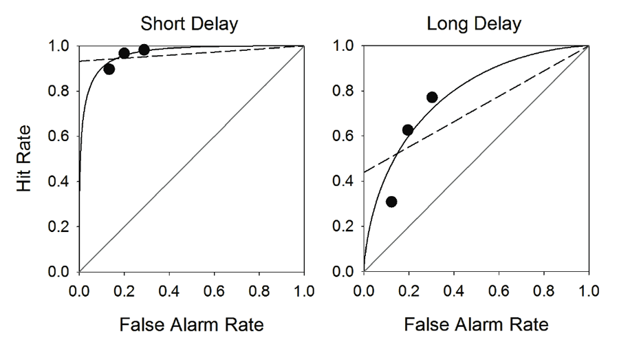
Figure 4. Empirical receiver operating characteristic (ROC) curves for two different retention intervals used in Experiment 3 of Wixted (1993). The short retention interval was 0.5 s (Short Delay), whereas the long retention interval was 12 s (Long Delay). Each graph depicts the hit rate vs. the false alarm rate for three reinforcement outcome conditions. The solid curves represent the best-fitting ROC functions based on signal-detection theory, whereas the dashed lines represent the best-fitting linear functions based on high-threshold theory.
The ROC data in this case were obtained by experimentally manipulating the birds’ decision criterion. In the neutral condition (the middle ROC point in each condition), the payoff for a correct “no-sample” decision was the same as the payoff for a correct “sample” decision. In both cases, the probability of food reinforcement for a correct response was .60. In the liberal condition (rightmost ROC point in each condition), the probability of food reinforcement was asymmetrical such that a correct sample choice was reinforced with probability 1.0, whereas a correct no-sample choice was reinforced with probability 0.20. These contingencies induced the birds to choose the sample alternative on a higher percentage of both sample and no-sample trials, thereby increasing both the hit rate and the false alarm rate relative to the neutral condition. To put this another way (and to make the results more relatable to the later discussion of eyewitness memory), the birds were more inclined to choose the sample alternative even when they were not especially confident that the sample had been presented. In the conservative condition (leftmost ROC point in each condition), the probability of food reinforcement was asymmetrical in the other direction such that a correct sample choice was reinforced with probability .20, whereas a correct no-sample choice was reinforced with probability 1.0. These contingencies induced the birds to choose the no-sample alternative on a higher percentage of both sample and no-sample trials, thereby decreasing both the hit rate and the false alarm rate relative to the neutral condition. In other words, the birds would only choose the sample alternative (with a payoff probability of only .20) when they were highly confident that the sample had in fact been presented on that trial. This would only occur if the memory strength on that trial were strong enough to exceed the high setting of the decision criterion.
The empirical ROC data are obviously closer to what the signal-detection model predicts than what the high-threshold model predicts. The same result is almost always observed on human memory tasks as well. As a result, signal-detection theory is generally regarded as the dominant account of human recognition memory, and d′ has become the standard dependent measure. This discriminability measure is essentially the same as log d in the Davison-Tustin (1978) model. Note that variations of the discrete-state high-threshold model can be found that will accommodate curvilinear ROC data, but my only purpose thus far has been to illustrate basic conceptual distinctions that separate the signal-detection view of memory from alternative theoretical views and to illustrate how the effort to test competing theoretical views brings one to ROC analysis.
To the Courtroom
The battle between high-threshold and signal-detection accounts of recognition memory has also played out (and in one form or another continues to play out) in the basic human memory literature. Although it sometimes seems like an abstract debate of interest only to math modelers, an argument could be made that a detailed inquiry into the underlying theoretics of recognition memory serves to underscore critical distinctions that are easily overlooked when the focus shifts to recognition memory in the real world (such as eyewitness memory). A critical distinction in the analyses considered above, and as noted earlier, is the well-known distinction between discriminability and response bias. In the high-threshold model, these two properties are captured by p and g, respectively, and in the signal-detection model, they are captured by d′ and c, respectively. Although the details of both models cannot simultaneously be true, the distinction they both draw between discriminability and response bias is similar and is far more important than it might seem to be at first glance. To see why, I turn next to the issue of the reliability of eyewitness identification and to the lab-based recognition memory tasks that are most commonly used to investigate it. For decades, this research has been mostly carried out without regard for the distinction between discriminability and response bias (for some notable exceptions, see Ebbesen & Flowe, 2002; Horry, Palmer, & Brewer, 2012; Meissner, Tredoux, Parker, & MacLin, 2005; Palmer & Brewer, 2012), and the reported results have had a profound effect on practices in the legal system. Without the guidance of basic theories of recognition memory (theories that protect one from compelling but often faulty intuitions), the argument can be made that eyewitness identification researchers got it wrong in several ways (Gronlund, Mickes, Wixted, & Clark, 2015).
From my perspective, this is a story about how basic psychological science and applied psychological science have drifted much too far apart from one another in recent years. As a result, mistakes have been made. My point is certainly not that eyewitness ID researchers got everything wrong, or that all eyewitness ID researchers made the influential mistakes I review next. The issues that the field got right (e.g., that memory is malleable and that eyewitness identification tests should not be biased against a suspect) are not controversial and are also not uniquely informed by signal-detection theory and ROC analysis. By contrast, the ones that the field got wrong are uniquely informed by signal-detection theory and ROC analysis, and those are the issues I focus on here.
Eyewitness Misidentification in the Real World
Many people, including, I would guess, most readers of this article, believe that eyewitness memory is inherently unreliable. And why not? Of the 334 wrongful convictions that have been overturned to date by DNA evidence since 1989, more than 70% were attributable, at least in part, to eyewitness misidentification (Innocence Project, 2015). A statistic like that is hardly a testimony to the impressive reliability of eyewitness identification. Instead, it seems like an obvious testimony to the catastrophic unreliability of eyewitness identification.
How can such tragic errors be reduced? For more than 30 years, applied psychological science has been brought to bear on this issue by using mock-crime laboratory studies. In a typical mock-crime study, participants (e.g., undergraduates) witness a mock crime (e.g., by watching a video of someone committing a crime, such as snatching a purse) and are later shown a photo lineup in which the perpetrator (the target) is either present or absent. A target-present lineup includes the perpetrator along with (usually five) similar fillers; a target-absent lineup is the same except that the perpetrator is replaced by another similar filler, as illustrated in Figure 5. That replacement filler can be designated as the innocent suspect. Note that not all studies pre-designate an innocent suspect in target-absent lineups, which adds complexity to the analysis of the data without changing anything of substance. Thus, in what follows, I shall assume that both target-present and target-absent lineups always have one suspect and five fillers, as real-world lineups typically do. Just as in a real-world investigation, a witness presented with a photo lineup in a mock-crime study can (a) identify a suspect (a suspect ID of an innocent or a guilty individual), (b) identify a filler (a filler ID), or (c) reject the lineup (no ID).
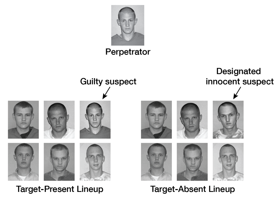
Figure 5. In a typical mock-crime study, participants view a simulated crime committed by a perpetrator and are later tested with either a target-present lineup (containing a photo of the perpetrator and five similar fillers) or a target-absent lineup in which the photo of the perpetrator has been replaced by the photo of another filler. In this example, the individual depicted in the replacement photo serves the role of the innocent suspect. In this type of study, mistakenly identifying the innocent “suspect” has traditionally been the error of most interest.
A suspect ID is the most consequential outcome of a lineup procedure because, as a general rule, only suspects who are identified from a lineup are placed at risk of prosecution. A suspect ID from a target-present lineup rightfully imperils the guilty perpetrator, but a suspect ID from a target-absent lineup wrongfully imperils an innocent suspect. A mistaken filler ID does not imperil anyone because the fillers are known to be innocent (e.g., the fillers might be database photos of people imprisoned in another state). The two key dependent measures in a mock-crime study are the correct ID rate (proportion of target-present lineups from which the guilty suspect is identified) and the false ID rate (proportion of target-absent lineups from which the innocent suspect is identified). In other words, this is a recognition task in which the hit rate and the false alarm rate are measured. Therefore, one’s thoughts should already be turning to signal-detection theory and ROC analysis, but many years went by (and extensive reforms were made to the legal system) before the first eyewitness ROC analysis was ever performed.
Simultaneous vs. Sequential Lineups in the Lab.
In light of the DNA exoneration cases, a major goal of scientific research (understandably) has been to find ways to reduce the false ID rate without appreciably reducing the correct ID rate. One simple change in the way that photo lineups are administered has long been thought to help protect innocent suspects from being mistakenly identified without much cost in terms of correctly identifying guilty suspects. Specifically, instead of presenting all six photos simultaneously (the traditional approach, as illustrated in Figure 5), the lineup photos are presented sequentially (one at a time) for individual yes/no decisions (Lindsay & Wells, 1985). The test effectively stops when someone is identified as the perpetrator. If the sequential test continues beyond that point, only the first identification typically counts (second laps are usually not allowed in lab studies, though they tend to be allowed in real-world sequential lineups).
Mock-crime studies have often found that sequential lineups result in a lower false ID rate. These same studies have often found that sequential lineups also lower the correct ID rate but to a lesser extent. In a review of the literature, Steblay, Dysart, and Wells (2011) reported that the average HR and FAR for the simultaneous lineup procedure equal 0.52 and 0.28, respectively, whereas the corresponding values for the sequential lineup procedure equal 0.44 and 0.15, respectively. Thus, on average, the sequential procedure yields both a lower HR and a lower FAR—an ambiguous outcome in terms of identifying the better procedure. Still, the drop in the FAR exceeds the drop in the HR. To the untrained eye, that seems to suggest a sequential superiority effect.
In an effort to quantify the diagnostic accuracy of the competing lineup procedures in terms of a single measure, eyewitness identification researchers have long relied on a statistic known as the diagnosticity ratio (correct ID rate ∕ false ID rate). Although the issue is contested (e.g., Clark, 2012; Gronlund, Carlson, Dailey, & Goodsell, 2009), some meta-analytic reviews of the mock-crime literature have concluded that the diagnosticity ratio is generally higher for sequential lineups (Steblay, Dysart, Fulero, & Lindsay, 2001; Steblay et al., 2011). For example, using the numbers reported by Steblay et al. (2011), the diagnosticity ratio for the sequential lineup procedure (0.44 ∕ 0.15 = 2.93) is higher than that of the simultaneous lineup procedure (0.52 ∕ 0.28 = 1.86), which led them to conclude that the sequential procedure is superior. The diagnosticity ratio increases because, when switching to the sequential procedure, the proportional drop in the FAR exceeds the proportional drop in the HR. That in itself seems like a positive outcome, thereby favoring the sequential procedure. The case in favor of the sequential procedure seems even more secure when one considers what the diagnosticity ratio actually measures. If half the lineups are target-present lineups and half are target-absent lineups (which is true of most of the relevant studies), then the diagnosticity ratio is a direct measure of the posterior odds of guilt. If the sequential procedure yields a higher diagnosticity ratio, then not only is the FAR rate lower, the posterior odds that an identified suspect is actually guilty are higher (i.e., the ID is more trustworthy) compared to a suspect identified from a simultaneous lineup. On the surface, the case in favor of the sequential procedure seems very strong indeed. Based on this interpretation of the empirical literature, approximately 30% of law enforcement agencies in the United States that use photo lineups have now adopted the sequential procedure (Police Executive Research Forum, 2013). Not many areas of psychological research can rival the real-world impact that eyewitness identification research has had.
Note that when using a lineup procedure, the essence of the task is to discriminate between innocent and guilty suspects. It is a detection task in much the same way that a sample/no-sample task with a pigeon is. It seems trickier because of the presence of fillers (what should one do with a filler ID?), but fillers have not stood in the way of computing the hit and false alarm rates that have convinced many that sequential lineups are diagnostically superior to simultaneous lineups. If there are 100 target-present lineups, and witnesses (a) identify the suspect in 52 of the lineups, (b) identify a filler in 16 of the lineups, and (c) reject the remaining 32 lineups, the hit rate is 52 ∕ 100 = .52. Similarly, if there are 100 target-absent lineups, and witnesses (a) identify the suspect in 24 of the lineups, (b) identify a filler in 32 of the lineups, and (c) reject the remaining 44 lineups, the false alarm rate is 24 ∕ 100 = .24. Thus, filler IDs are not typically counted when computing hit and false alarm rates (nor should they be). Ideally, the goal is to get the FAR as close to 0 as possible and the HR as close to 1.0 as possible. In other words, the goal is to maximize discriminability between innocent and guilty suspects. The sequential lineup procedure seems to do a good job of reducing the FAR without compromising the HR too much (though it would be better if it actually increased rather than slightly decreasing the HR). It may seem as if the data suggest that sequential lineups achieve the goal of increasing discriminability, but consider for a moment the fact that, so far, a compelling story in favor of the sequential procedure has been told with no mention of a measure of discriminability (and with no look at the ROC).
As discussed earlier in connection with high-threshold theory vs. signal-detection theory, a singular pair of hit and false alarm rates does not characterize the discriminability of a procedure. Instead, the whole ROC does. To say that the goal is to maximize discriminability is to say that the goal is to achieve the highest possible ROC. The ROC depicts the family of achievable hit and false alarm rates associated with a particular condition. If Condition A yields a higher ROC than Condition B, it means that both states of the world can be more accurately categorized in Condition A compared to Condition B. That is, if it yields a higher ROC, Condition A is capable of achieving both a higher HR and a lower FAR than Condition B.
Instead of performing ROC analysis, researchers in the field of eyewitness identification computed the diagnosticity ratio for each condition in an effort to determine which lineup format is superior. The problem is that this intuition-based approach cannot reveal the diagnostically superior condition when the HR and FAR both change in the same direction (which is the case here: the HR and the FAR are both lower for the sequential procedure). Why not? The reason why a higher diagnosticity ratio does not identify the superior procedure is most easily appreciated by examining a basic property of an ROC curve. Keep in mind that an ROC shows the full range of hit and false alarm rates that are achievable as response bias ranges from liberal to conservative (while holding discriminability constant). An important consideration that has only recently come to be understood in the field of eyewitness identification is that a natural consequence of more conservative responding (in addition to the fact that the correct and false ID rates decrease) is that the diagnosticity ratio increases (Gronlund, Wixted, & Mickes 2014; Wixted & Mickes, 2012, 2014). Critically, this occurs whether more conservative responding is induced for the simultaneous procedure (e.g., using instructions that encourage eyewitnesses not to make an ID unless they are confident of being correct) or more conservative responding is induced by switching to the sequential procedure. The diagnosticity ratio continues to increase as responding becomes ever more conservative, all the way to the point where both the correct and false ID rates approach 0, in which case administering a lineup would be practically useless even though the diagnosticity ratio would be very high (Wixted & Mickes, 2014). Thus, achieving the highest possible diagnosticity ratio by inducing ever more conservative responding is not a logical goal to pursue.
As noted by a recent National Academy committee report on eyewitness identification, “ROC analysis represents an improvement over a single diagnosticity ratio” (National Research Council, 2014, p. 80). To be sure, the committee did not judge ROC analysis to be such a flawless methodology that the field can now stop worrying about the best way to compare lineup procedures and use ROC analysis forevermore. Instead, the committee also expressed reservations about confidence-based ROC analysis because different eyewitnesses might exhibit differences in the inclination to express a certain level of confidence, such as high confidence. That is, the memory strength that warrants high confidence for one eyewitness might warrant only medium or low confidence for another. Thus, although the committee agreed that ROC analysis represents an advance over the diagnosticity ratio, it also called for new research to identify even better diagnostic methodologies. For the time being, however, there are only two choices: the diagnosticity ratio and ROC analysis. Given that choice, ROC analysis is clearly the better option. This is an important point to consider because the two approaches (namely, the diagnosticity ratio vs. ROC analysis) can yield opposite answers to the question of which lineup procedure is diagnostically superior.
To appreciate the advantage of ROC analysis, consider the two ROC curves illustrated in Figure 6. The ROC is a plot of the family of hit and false alarm rates (i.e., correct and false ID rates) associated with each procedure, and values shown next to each data point indicate the diagnosticity ratio (i.e., correct ID rate ∕ false ID rate) for that point. In this example, Procedure A is diagnostically superior to Procedure B because for any given false ID rate, Procedure A can achieve a higher correct ID rate. If only a single ROC point is computed for each procedure and those two points are then compared using the diagnosticity ratio (as was done in the vast majority of mock-crime lab studies comparing simultaneous and sequential lineups), the diagnostically inferior lineup procedure could be misconstrued as being the superior procedure (e.g., imagine computing only the rightmost ROC point for each procedure and comparing them using the diagnosticity ratio). The only way to determine the diagnostically superior procedure is to trace out the ROC (i.e., trace out the obtainable hit and false alarm rates) for each lineup procedure.
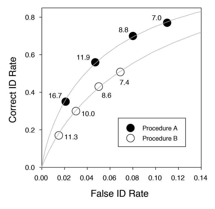
Figure 6. Illustration of receiver operating characteristic plots for two hypothetical lineup procedures. Each lineup procedure is constrained to yield correct and false ID rates that fall on a curve as responding changes from being very conservative (lower leftmost point of each procedure) to being very liberal (upper rightmost point for each procedure). Values shown next to each data point indicate the diagnosticity ratio (correct ID rate ∕ false ID rate) for that point. In this example, Procedure A is diagnostically superior to Procedure B because for any given false ID rate, Procedure A can achieve a higher correct ID rate. If only a single ROC point is computed for each procedure and the procedures are then compared using the diagnosticity ratio (as was done in the vast majority of mock-crime lab studies comparing simultaneous and sequential lineups), the diagnostically inferior lineup procedure could be misconstrued as being the superior procedure (e.g., imagine computing only the rightmost ROC point for each procedure and comparing them using the diagnosticity ratio).
The easiest and by far the most common way to construct an ROC in experiments with humans is to collect confidence ratings. The overall hit and false alarm rates (i.e., the values that are usually reported as the correct and false ID rates) are computed using all correct suspect IDs from target-present lineups and all incorrect suspect IDs from target-absent lineups. In the example given above, there were 52 correct suspect IDs from 100 target-present lineups (made with varying degrees of confidence) and 24 incorrect suspect IDs from 100 target-absent lineups (again made with varying degrees of confidence). This yielded overall hit and false alarm rates of .52 and .24 respectively. ROC analysis essentially gives you permission to disregard suspect IDs that are made with low confidence (as the legal system might do). If you disregard low-confidence suspect IDs by treating them as effective non-IDs, then (a) you have adopted a more conservative standard for counting suspect IDs, and (b) you will have fewer correct and false IDs than you did before, so the correct and false ID rates will now both be lower. Imagine that two correct suspect IDs were made with low confidence and 10 incorrect suspect IDs were made with low confidence. Excluding these IDs leaves 52 – 2 = 50 correct suspect IDs from 100 target-present lineups and 24 – 10 = 14 incorrect suspect IDs from 100 target-absent lineups. Thus, the new hit and false alarm rates are .50 and .14, respectively. Now there are two points to plot on the ROC. When all IDs are counted regardless of confidence, the resulting correct and false ID rates correspond to the rightmost ROC point. Disregarding low-confidence IDs yields the next ROC point down and to the left.
Once you realize that you are not obligated to count IDs made with low confidence, it immediately follows that you are also not obligated to count IDs made with medium confidence. Excluding IDs made with low or medium confidence by treating them as effective non-IDs yields yet another pair of correct and false ID rates (i.e., another ROC point, again down and to the left). Critically, as noted above, the diagnosticity ratio increases monotonically as an ever-higher confidence standard is applied. Although it is easy to imagine that the diagnosticity ratio might not increase as responding becomes more conservative, it invariably occurs and is naturally predicted by signal-detection theory (see Appendix of Wixted & Mickes, 2014).
The point is that one must perform ROC analysis, not compute the diagnosticity ratio from a singular pair of hit and false alarm rates, to identify the diagnostically superior lineup procedure. The first ROC study of eyewitness identification procedures only appeared in late 2012 and it is reproduced here in Figure 7 (Mickes, Flowe, & Wixted, 2012). The results came as a surprise because they unexpectedly revealed a simultaneous superiority effect. Before that study was performed, there had not been a single suggestion that simultaneous lineups might be superior to sequential lineups. Instead, over the years, the debate had been whether there was a sequential superiority effect (because it tended to yield a higher diagnosticity ratio) or whether the two procedures were diagnostically equivalent. Now, multiple ROC studies of simultaneous vs. sequential lineups have been published, and they all show evidence of a simultaneous superiority effect, though the effect is not always significant (Carlson & Carlson, 2014; Dobolyi & Dodson, 2013; Gronlund et al., 2012; Mickes et al., 2012). To date, no ROC study has shown the slightest hint of a sequential superiority effect.
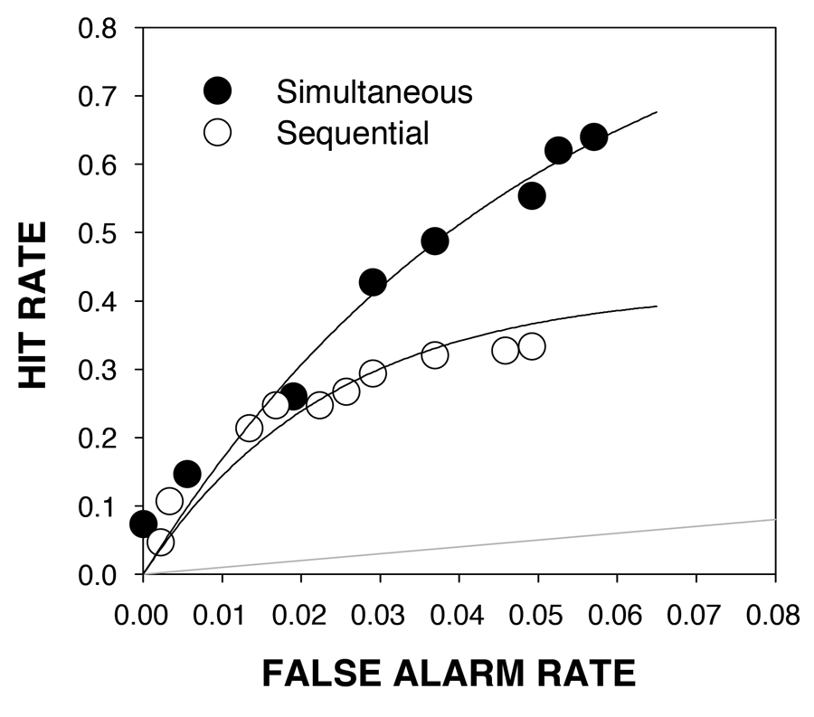
Figure 7. Confidence-based receiver operating characteristics (ROCs) from an experiment in which memory for a perpetrator in a simulated crime was tested using either a simultaneous lineup procedure (filled symbols) or a sequential lineup procedure (open symbols). The participants were undergraduates tested in a laboratory, and fair lineups were used. The solid gray line represents chance performance.
Simultaneous vs. Sequential Lineups in the Real World
Do the ROC results from lab studies generalize to the real world? In two recent police department field studies comparing the two lineup formats (one in Austin, Texas, and the other in Houston, Texas), evidence of a simultaneous superiority effect was observed. Using expert ratings of incriminating evidence against identified suspects, Amendola and Wixted (2015) found that, in Austin, the results significantly favored the simultaneous procedure. In other words, the results suggested that guilty suspects were more likely to be identified—and innocent suspects were less likely to be misidentified—using simultaneous lineups compared to sequential lineups. Similarly, in the Houston field study, Wixted, Mickes, Clark, Dunn, & Wells (in press) again found evidence of a simultaneous superiority effect based on police officer ratings of incriminating evidence against identified suspects. The effect was not always significant, depending on how the data were analyzed, but the trend was always in a direction that favored the simultaneous procedure. In addition, a separate signal-detection-based analysis of eyewitness confidence ratings in the Houston field study also favored the simultaneous procedure.
ROC analysis cannot be performed on data collected from real eyewitnesses because one does not know whether suspect IDs are correct or incorrect (information that is needed to compute the correct and false ID rates that make up the ROC). Instead, as noted above, the lineup performance measure used in these two police department field studies was “independent evidence of guilt,” which is a proxy for odds of guilt. This measure is conceptually identical to the diagnosticity ratio that has been used in lab studies for years. That is, the diagnosticity ratio—correct ID rate ∕ false ID rate—is also an odds-of-guilt measure. That fact raises an obvious question: Why is it acceptable to use an odds-of-guilt measure for real eyewitnesses when it is not acceptable to use it for lab studies?
An odds-of-guilt measure is problematic only when responding is more conservative for one lineup procedure than the other. In lab studies, sequential lineups often induce more conservative responding. Under those conditions, an odds-of-guilt measure like the diagnosticity ratio would be expected to favor the more conservative procedure whether or not it is the diagnostically superior procedure because that measure increases as responding becomes more conservative. However, in both police department field studies (the one conducted in Austin and the one conducted in Houston), responding happened to be similarly biased for simultaneous and sequential lineups in the sense that IDs were made with approximately equal frequency for both lineup types. Under those conditions only, an odds-of-guilt measure correctly identifies the diagnostically superior lineup procedure. In both police department field studies, the simultaneous procedure was favored according to the odds-of-guilt measure, just as would be predicted from recent lab-based ROC analyses.
Pushback from Proponents of the Sequential Procedure
Perhaps understandably, longstanding advocates of the sequential procedure have a different take on the data. For example, Wells, Steblay, & Dysart (2015a) argued that the results of the Austin Police Department field study, when combined with police department field data from three other study sites (San Diego, California; Tucson, Arizona; and Charlotte-Mecklenburg, North Carolina), actually favored the sequential procedure. Their argument was based not on independent incriminating evidence against identified suspects (as our analyses were) but was instead based on the fact that the filler ID rate for sequential lineups was lower than the filler ID rate for simultaneous lineups. Because fillers are known to be innocent, the interpretation was that sequential lineups better protect innocent suspects from being misidentified.
In addition, Wells, Steblay, and Dysart (2015b) and Steblay, Dysart, and Wells (2015) argued that the sample of identified suspects studied by Amendola and Wixted (2015) was, for unidentified reasons, biased against the sequential procedure. The basis of their concern about a possibly biased sample was that the ultimate case outcomes (i.e., proportion of suspects ultimately found guilty by jury or plea bargain) differed noticeably for the suspects identified in Austin (where our expert ratings study was conducted) compared to suspects identified in all four study sites aggregated together (Austin, Charlotte-Mecklenburg, San Diego, and Tucson). In Austin, the results showed that a higher proportion of suspects identified from simultaneous lineups was found guilty compared to sequential lineups; in the full data set, by contrast, the case outcomes for simultaneous and sequential lineups were more evenly balanced. Their interpretation of this pattern of data was that, for some reason, the Austin sample included an unusually high number of guilty suspects in the simultaneous condition. If so, it would not be surprising that independent expert ratings of guilt would also be higher for the simultaneous sample than for the sequential sample.
A subsequent analysis by Amendola and Wixted (2015) showed that the case made by Wells and colleagues, which is dependent on aggregating data across study sites, overlooks statistically significant evidence of site variance that effectively disallows aggregating data across sites. For example, based on an analysis of data aggregated across study sites, Wells et al. (2015a) argued that the lower filler ID rate observed for sequential lineups suggests a sequential lineup advantage. However, by examining the data separately by study site, Amendola and Wixted (2015) showed that the observed filler ID rate difference (like the higher diagnosticity ratio often associated with sequential lineups in lab studies) is entirely attributable to a conservative response bias that was evident in the three non-Austin study sites—a response bias that was absent in the Austin study site. As with lab studies, the conservative response bias sometimes induced by sequential lineups does not indicate a sequential superiority effect. Moreover, this previously unappreciated evidence of site variance also accounts for why Wells et al. (2015b) and Steblay et al. (2015) came to believe that the Amendola and Wixted (2015) sample was biased against the sequential procedure. As noted above, the basis of their concern about a possibly biased sample was that the case outcomes (i.e., proportion ultimately found guilty) for the suspects identified from lineups in Austin differed noticeably from the case outcomes for the suspects identified from lineups aggregated across all four study sites. However, given evidence of site variance, there is no reason why the Austin sample (where no conservative response bias was observed for sequential lineups relative to simultaneous lineups) should be representative of the data collapsed across study sites. Moreover, because response bias was similar for simultaneous and sequential lineups in the Austin sample only, any comparison of lineup performance based on incriminating evidence of guilt has to be limited to data from that site alone. For the Austin data, filler ID rates show no hint of a sequential superiority effect, and the Amendola and Wixted (2015) expert ratings data show clear evidence of a simultaneous superiority effect.
Theoretical Basis of the Simultaneous Superiority Effect.
In retrospect, the diagnostic advantage of simultaneous lineups should not have come as a surprise. The reason is that no theoretical explanation as to why sequential lineups might yield higher discriminability has ever been advanced, and the longstanding absence of a theoretical explanation to that effect probably should have been a cause for concern. To be sure, there is a prominent theory about why different patterns of responding are maintained by simultaneous and sequential lineups, but it is not a theory of discriminability. This well-known theory draws a distinction between absolute and relative decision strategies (Lindsay & Wells, 1985; Wells, 1984). According to this account, simultaneous lineups encourage a witness to identify the lineup member who most resembles the eyewitness’s memory of the perpetrator (a relative decision strategy). By contrast, sequential lineups encourage a witness to choose a lineup member only if the familiarity signal exceeds an absolute decision criterion. Wixted and Mickes (2014) argued that this is a theory of response bias (i.e., simultaneous lineups engender a more liberal response bias than sequential lineups), not a theory of discriminability. In agreement with this view, Wells (1984) wrote, “It is possible to construe of the relative judgments process as one that yields a response bias, specifically a bias to choose someone from the lineup” (p. 94).
But what about discriminability—that is, the ability to tell the difference between innocent and guilty suspects? Until recently, no theory of discriminability for the lineup task had ever been proposed. A case could be made that a theory of response bias in terms of absolute and relative responding is much less important than a theory of discriminability because manipulating response bias is easy to do using either kind of lineup procedure (i.e., one need switch lineup procedures to influence response bias). By contrast, in the absence of theoretical guidance, improving discriminability is hard. Fortunately, simple theoretical principles from the perceptual learning literature very naturally explain why simultaneous lineups should be diagnostically superior to sequential lineups in terms of discriminability. The basic idea, as argued by Wixted and Mickes (2014), is that simultaneous lineups immediately teach the witness that certain facial features are nondiagnostic and therefore should not be relied upon to try to decide whether or not the guilty suspect is in the lineup. The nondiagnostic features are the features that are shared by every member of the lineup (the fillers and suspect alike, and whether the suspect is innocent or guilty). These are the features that were used to select individuals for inclusion in the lineup—that is, features that match the physical description of the perpetrator. Because everyone in the lineup shares those features, relying on them to determine whether or not the guilty suspect is in the lineup can only harm discriminative performance. Simultaneous lineups immediately teach the witness what the nondiagnostic features are (namely, the features that are obviously shared by all six members of the lineup, such as the fact that they are all young white males), thereby allowing those features to be given less weight and, as a result, enhancing discriminative performance.
Again not surprisingly, longstanding advocates of the sequential procedure have taken issue not just with our interpretation of police department field study data but also with recent lab-based ROC analyses that confirmed the simultaneous superiority effect in terms of discriminability (e.g., Wells, Smalarz, & Smith, in press; Wells, Smith, & Smalarz, in press). In fact, they are taking the position that ROC analysis is not informative when it comes to comparing lineup procedures, declaring not only that I and other researchers are wrong about that but that so is the National Academy of Sciences committee that recently weighed in on the issue (National Research Council, 2014). In their view, the work that my colleagues and I performed on this issue misled the esteemed National Academy committee, thereby explaining why the committee made the mistake of endorsing ROC analysis over the diagnosticity ratio. As they put it: “Yes, the National Research Council (NRC) report got it wrong by interpreting ROC analyses on lineups as measures of underlying discriminability. But that is how the NRC eyewitness committee read and interpreted Wixted and Mickes’ work” (Wells, Smith, & Smalarz, in press). As part of an invited debate about these issues, Mickes and I have elaborated on the case in favor of ROC analysis (Wixted & Mickes, in press a; Wixted & Mickes, in press b). Lampinen (in press) recently joined the debate by arguing against the utility of ROC analysis.
It seems clear that the issue will continue to be debated in the years to come, but it is hard for me to imagine that the ultimate judgment will be that ROC analysis has nothing useful to offer. The mere fact that, in the past, researchers based their argument in favor of sequential lineups on the ratio of the correct ID rate to the false ID rate means that they already computed one point on the ROC. If there is a reasonable case to be made as to why it is mandatory to compute one point on the ROC to measure lineup performance yet is utterly inappropriate to examine any of the other points on the ROC, then that case should be made. Thus far, the anti-ROC arguments have avoided this basic consideration. Anyone interested in this topic would do well to read the various articles in this ongoing debate and then make their own judgment as to who has the stronger argument. The larger community of scientists will, of course, be the ultimate judge. To some extent, that is already happening (National Research Council, 2014; Rotello, Heit, & Dubé, 2015), and this is how it should be. For too long, some of the most influential applied research has been conducted by psychologists who are (in my view) too far removed from basic psychological science. Indeed, lineup format is not the only consequential issue that applied psychologists got wrong over the years. The other important issue where key mistakes have been made has to do with the very notion of eyewitness unreliability itself.
Eyewitnesses are nowhere near as unreliable as they have long been thought to be. As described in more detail below, eyewitness ID researchers have corrected this mistake with a compelling series of empirical calibration studies (most of which come from Neil Brewer and his colleagues), but the information seems almost exclusively confined to that small field. In my experience, the larger community of experimental psychologists typically reacts with shock in response to the claim that, under typical laboratory conditions (e.g., fair lineups, no administrator influence, etc.), eyewitness confidence is a strong indicator of reliability. Moreover, the earlier work suggesting that eyewitness identification is inherently unreliable even under pristine laboratory conditions has had a profound influence on the U.S. legal system, and that influence is growing, not shrinking. Courts across the land are increasingly inclined to disregard expressions of confidence made by eyewitnesses. A case can be made—and we do make the case—that this practice unnecessarily places innocent suspects at risk (exactly the opposite of what was intended).
Confidence and Accuracy
To many, the suggestion that eyewitnesses are not inherently unreliable may sound as implausible as the idea that ESP is real. However, my colleagues and I recently made the case that the blanket indictment of the reliability of eyewitness identification from a lineup is incorrect and serves only to place innocent suspects at greater risk of being wrongfully convicted (Wixted, Mickes, Clark, Gronlund, & Roediger, 2015). To appreciate why, it is essential to first draw a distinction between the initial eyewitness ID from a lineup and the much later ID that occurs at trial. There is nearly unanimous agreement that initial confidence can become artificially inflated for a variety of reasons such that by the time a trial occurs, an original ID made with low confidence (for example) can morph into an ID made with high confidence (Wells & Bradfield, 1998, 1999). The DNA exoneration cases that were associated with eyewitness misidentification involved high-confidence IDs of an innocent defendant made in front of a jury during a trial (and the jury interpreted the ID as compelling evidence of guilt). Errors like these make it clear that eyewitness identification can be unreliable under some conditions, such as at trial. Indeed, through decades of work, Loftus and her colleagues have established beyond any reasonable doubt that memory is malleable (Loftus, 2005; Loftus & Pickrell, 1995; Loftus & Palmer, 1974; Loftus, Miller, & Burns, 1978).
But is eyewitness memory always unreliable? The idea that eyewitness memory is generally unreliable (not just at trial) was set in stone by the fact that mock-crime studies once seemed to convincingly show that, even at the time of the initial identification from a lineup (long before a trial occurs and before memory contamination has much of an opportunity to take place), eyewitnesses who make a high-confidence identification are only somewhat more accurate than the presumably error-prone eyewitnesses who make a low-confidence identification (Devenport, Penrod, & Cutler, 1997). In other words, this research seemed to indicate that the relationship between confidence and accuracy is weak across the board.
The relationship between confidence and accuracy was originally measured by computing the standard Pearson r correlation coefficient between the accuracy of a response (e.g., coded as 0 or 1) and the corresponding confidence rating (e.g., measured using a five-point scale from “just guessing” to “very sure that is the person”). A correct response consists of (a) a suspect ID from a target-present lineup or (b) the rejection of a target-absent lineup, whereas an incorrect response consists of (a) a suspect ID from a target-absent lineup, (b) a filler ID from either type of lineup, or (c) the rejection of a target-present lineup. Because accuracy is coded as a dichotomous variable, the Pearson r in this case is known as a point-biserial correlation coefficient.
In an early review of the literature, Wells and Murray (1984) reported that the average point-biserial correlation between confidence and accuracy in studies of eyewitness identification was only .07 (declaring on that basis that confidence was “functionally useless” in forensic settings), but in a later meta-analysis, Sporer, Penrod, Read, and Cutler (1995) found that the relationship is noticeably stronger—about .41—when the analysis was limited to only those who make an ID from a lineup (i.e., when the analysis was limited to “choosers” who ID a suspect or a filler). Limiting the analysis to choosers is reasonable because only witnesses who choose someone would end up testifying in court against the suspect they identified. Still, even this higher correlation is generally viewed in a negative light. For example, Wilson, Hugenberg, and Bernstein (2013) recently stated that “. . . one surprising lesson that psychologists have learned about memory is that the confidence of an eyewitness is only weakly related to their recognition accuracy (see Sporer et al., 1995, for a review).” Thus, many still view the relationship between eyewitness confidence and accuracy as being of limited utility. In a well-known survey that is often cited in U.S. courts, Kassin, Tubb, Hosch, and Memon (2001) found that 90% of the respondents agreed with the following statement: “An eyewitness’s confidence is not a good predictor of his or her identification accuracy.” In addition, a recent amicus brief filed by the Innocence Project in Michigan states that “A witness’ confidence bears, at best, a weak relationship to accuracy.”
The problem with this conclusion is that it is based on a statistic that does not adequately characterize the relationship between confidence and accuracy (in much the same way that the diagnosticity ratio does not adequately characterize the diagnostic performance of a lineup procedure). Juslin, Olsson, and Winman (1996) definitively showed that, counterintuitively, a low correlation coefficient does not necessarily imply a weak relationship between confidence and accuracy. They argued that a better way to examine the relationship—the way that is more compatible with predictions made by signal-detection theory—would be to simply plot accuracy as a function of confidence.
Signal-Detection Predictions Concerning the Confidence–Accuracy Relationship
A key assumption of signal-detection theory is that a decision criterion is placed somewhere on the memory strength axis, such that an ID is made if the memory strength of a face (target or lure) exceeds it. The correct ID rate is represented by the proportion of the target distribution that falls to the right of the decision criterion, and the false ID rate is represented by the proportion of the lure distribution that falls to the right of the decision criterion. These theoretical considerations apply directly to eyewitness decisions made using a showup (i.e., where a single suspect is presented to the eyewitness), but they also apply to decisions made from a lineup once an appropriate decision rule is specified (Clark, Erickson & Breneman, 2011; Fife, Perry, & Gronlund, 2014; Wixted & Mickes, 2014). One simple lineup decision rule holds that eyewitnesses first determine the lineup member who most closely resembles their memory for the perpetrator and then identify that lineup member if subjective memory strength for that individual exceeds a decision criterion (see Clark et al. 2011 for a discussion of a variety of possible lineup decision rules).
Figure 8 shows how SDT conceptualizes confidence ratings associated with IDs that are made using a three-point scale (1 = low confidence, 2 = medium confidence, and 3 = high confidence). Theoretically, the decision to identify a target or a lure with low confidence is made when memory strength is high enough to support a confidence rating of 1 but is not high enough to support a confidence rating of 2 (i.e., when memory strength falls between the first and second decision criteria). Similarly, a decision to identify a target or a lure with the next highest level of confidence is made when memory strength is sufficient to support a confidence rating of at least 2 (but not 3). A high-confidence rating of 3 is made when memory strength is strong enough to exceed the rightmost criterion.
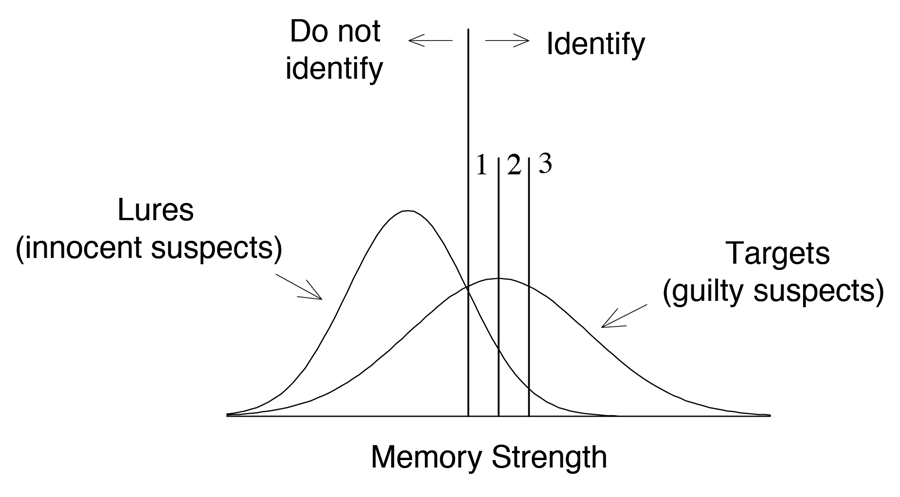
Figure 8. A depiction of the standard Unequal-Variance Signal-Detection (UVSD) model for three different levels of confidence, low (1), medium (2), and high (3). An unequal-variance model is depicted here because the results of list-memory studies are usually better modeled by assuming unequal rather than equal variance. Whether this is also true of lineup studies is not yet known.
In this illustrative example, 37% of targets would be associated with memory strengths that exceed the highest confidence criterion (Figure 9, top left panel). By contrast, only about 2% of lures would be associated with memory strengths that exceed the highest confidence criterion (Figure 9, top right panel). If innocent and guilty suspects appeared equally often (i.e., if we assume equal base rates), this would mean that 37 out of 39 high-confidence IDs would be correct. Thus, the proportion correct for high-confidence IDs would be 37 ∕ (37 + 2) = .95.
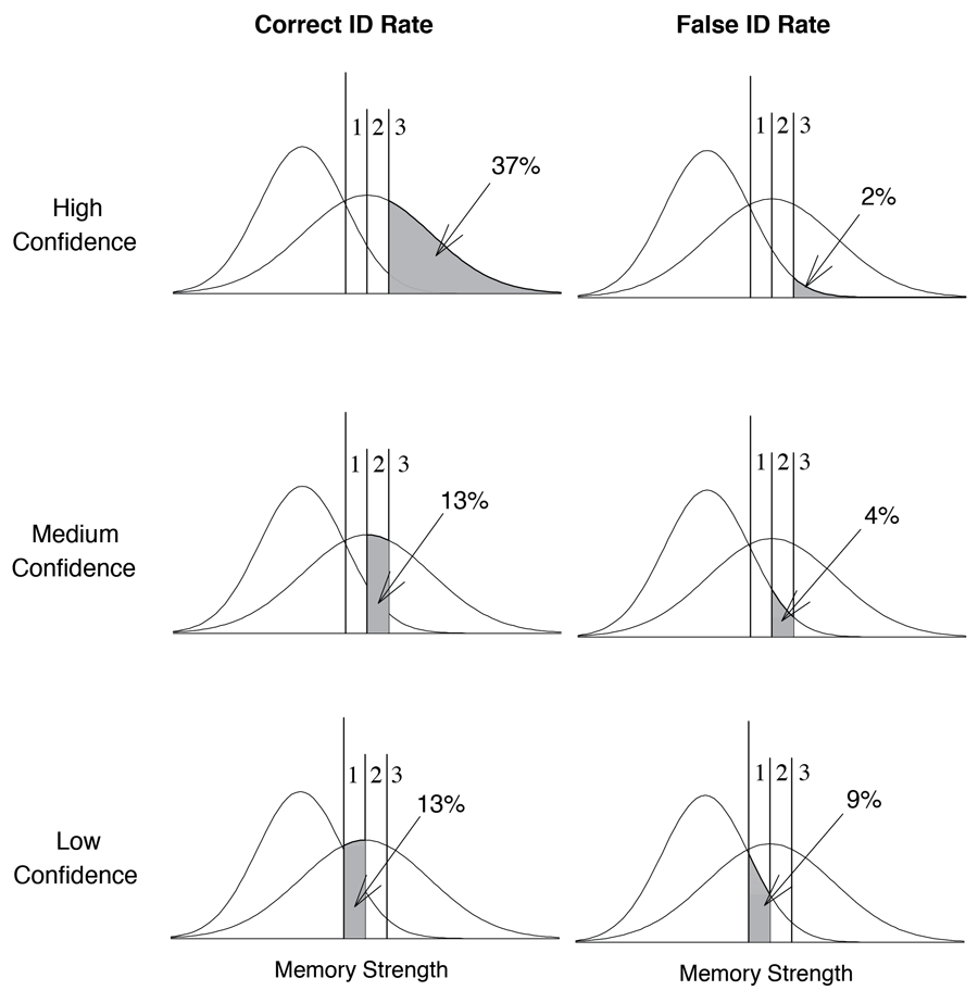
Figure 9. Signal-detection-based interpretation of correct ID rates (left panels) and false ID rates (right panels) for high-confidence (top), medium-confidence (middle), and low-confidence (bottom) IDs.
Next, consider IDs made with medium confidence (a rating of 2 on the 1-to-3 confidence scale). Only 13% of targets in this example would be associated with memory strengths that fall above the criterion required to receive a confidence rating of 2 but below the criterion required to receive a high-confidence rating of 3 (Figure 9, middle left panel), whereas about 4% of lures would be associated with memory strengths that fall in that same range (Figure 9, middle right panel). Thus, the proportion correct for medium-confidence decisions is 13 ∕ (13 + 4) = .76.
Finally, 13% of targets in this example would be associated with memory strengths that fall above the criterion required to receive a low-confidence rating of 1 but below the criterion required to receive a medium-confidence rating of 2 (Figure 9, bottom left panel), whereas about 9% of lures would be associated with memory strengths that fall in that same range (Figure 9, bottom right panel). Thus, the proportion correct for low-confidence decisions drops even further to 13 ∕ (13 + 9) = .59.
Figure 10 is a graph of proportion correct versus confidence for the hypothetical example illustrated above. Obviously, SDT predicts a strong relationship between confidence and accuracy. The details of what the theory predicts will vary from case to case, but so long as the target distribution is shifted to the right of the lure distribution (i.e., so long as a diagnostic memory signal exists) and so long as the confidence criteria are monotonically arranged on the memory strength axis, the theory predicts that confidence and accuracy will be positively related, and this is true even if the correlation coefficient, as typically computed, is low.
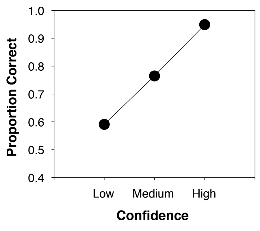
Figure 10. Predicted relationship between proportion correct and confidence for the signal-detection model illustrated in Figure 9.
Empirical Plots of the Confidence–Accuracy Relationship
A considerable body of research conducted in the time since the Sporer et al. (1995) review appeared has used a calibration approach (in which accuracy is plotted as a function of confidence measured using a 100-point scale), which is closer to how a signal-detection approach suggests that the data should be plotted (Figure 10). This body of research has almost always reported visually obvious evidence of a strong relationship between confidence and accuracy (Brewer & Wells, 2006; Brewer, Keast, & Rishworth, 2002; Palmer, Brewer, Weber, & Nagesh, 2013; Sauer, Brewer, Zweck, & Weber, 2010; Sauerland & Sporer, 2009; Brewer & Palmer, 2010; Weber & Brewer, 2004, 2006). This work explains why many eyewitness ID researchers no longer believe that confidence is, at best, a weak indicator of accuracy. Still, many do, and their views increasingly win the day in the U.S. legal system.
The dependent variable in a calibration analysis is an accuracy score of the general form correct IDs ∕ (correct IDs + incorrect IDs). If there were no incorrect IDs, then this measure would equal 1.0. If there were as many incorrect IDs as correct IDs, then it would equal .50. However, there is more than one way to compute a calibration accuracy score, depending on whether or not filler IDs are counted as incorrect IDs. Should filler IDs and innocent suspect IDs alike be counted as errors, or should only innocent suspect IDs be counted as errors?
Wixted et al. (2015) argued that for the information to be maximally informative to the legal system, filler IDs should not be included in the calculations (just as they are often not included when computing correct and false ID rates for diagnosticity ratio or ROC analyses). The eyewitness ID cases that end up before judges and juries are limited to identified suspects, and the question asked by the court is this: what does confidence tell us about the reliability of the suspect ID? Note that this is a question about the cases that go forward to prosecution using eyewitness identification as direct evidence of the suspect’s guilt, not about the full set of cases involving eyewitness who choose fillers or reject lineups. The accuracy of witnesses who identify suspects are of special interest, so the accuracy score of interest is guilty suspect IDs ∕ (guilty suspect IDs + innocent suspect IDs).
Although calibration studies typically count filler IDs as errors in their accuracy score (thereby lowering the accuracy score from what it would otherwise be), it is worth examining data from a representative study to see what suspect ID accuracy typically looks like as a function of confidence. A representative study by Dobolyi and Dodson (2013) can be used for this purpose. This was a face memory study in which the participating eyewitnesses were later tested using a six-person simultaneous or sequential photo lineup, and confidence ratings were taken using a 0-to-100 scale. The relationship between suspect ID accuracy and confidence—estimated from their data and collapsed across conditions—is shown in Figure 11. The results indicate that even low-confidence suspect IDs are fairly accurate (about 70% correct), though the 30% error rate would obviously be too high to justify a conviction based on a low-confidence ID alone. Remarkably, high-confidence suspect ID accuracy is almost perfect. These results are not atypical, though it is not uncommon to find high-confidence suspect ID accuracy to be closer to .95 than 1.0 (Wixted et al., 2015).
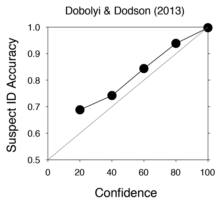
Figure 11. Suspect ID accuracy, which is equal to correct suspect IDs ∙ (correct suspect IDs + incorrect suspect IDs), for a lineup study reported by Dobolyi and Dodson (2013). This study used fair lineups with no designated innocent suspect, so incorrect suspect IDs were estimated by dividing the number of filler IDs from target-absent lineups by the lineup size of 6.
What data like these suggest is that the impression created by an earlier era of research that relied on the point-biserial correlation coefficient was misleading (suggesting, as it did, a weak confidence–accuracy relationship) and that the actual confidence–accuracy relationship is much more in line with what one would expect using signal detection as a guide. Unfortunately, the legal system increasingly accepts the idea that there is a weak correlation between confidence and accuracy, and jurors are increasingly encouraged to ignore expressions of eyewitness confidence (including initial confidence). If the relationship between eyewitness confidence and accuracy is initially strong, then an argument could be made that encouraging juries to disregard confidence places innocent suspects at increased risk of wrongful conviction. In his 2011 book Convicting the Innocent: Where Criminal Prosecutions Go Wrong, Brandon Garrett (2011a) analyzed trial materials for 161 DNA exonerees who had been misidentified by one or more eyewitnesses in a court of law. A key finding was that “. . . in 57% of these trial transcripts (92 of 161 cases), the witnesses reported that they had not been certain at the time of their earlier identifications” (p. 49, emphasis in original). Information about the initial confidence for the remaining 43% of cases was not available.
Figure 11 suggests that an expression of low confidence is how eyewitnesses communicate the fact that the ID they are making carries a high risk of being wrong. In fact, the DNA exoneration cases suggest that this is as true of the real world as it is of the laboratory. An initial ID made with low confidence is a red flag that the risk of eyewitness misidentification is high. Therefore, teaching jurors to ignore confidence is teaching them to ignore a critical clue that the identified suspect may be innocent. No fewer than 57% of DNA exonerees were convicted based on low-confidence initial IDs that later morphed into high-confidence IDs due to the malleability of memory. If it were understood that initial confidence (and only initial confidence) is clearly diagnostic of guilt, then many of these individuals might never have been convicted in the first place. Note that this is even true of what is perhaps the most famous case of eyewitness misidentification, the one that is usually used to illustrate how unreliable eyewitness identification can be. During a trial that was held in 1985, Jennifer Thompson confidently identified Ronald Cotton as the man who had raped her. Cotton was convicted largely on the basis of her testimony, but he was later exonerated by DNA evidence after spending more than 10 years in prison. Long before the trial, however, Thompson’s initial identification of Cotton from a photo lineup was characterized by a prolonged period of hesitation and indecision that lasted for nearly five minutes and that ended with a low-confidence verbal identification consisting of the words “I think this is the guy” (p. 33, Thompson-Cannino, Cotton, & Torneo, 2009; Garrett, 2011b). However, after confirmatory feedback from the police, Thompson quickly became confident that Cotton was the rapist. Her initial lack of confidence spoke volumes, but no one paid attention to it.
The same pattern continues to be seen in DNA exoneration cases. A new DNA exoneration case was in the news as this paper was being prepared for submission. The article says: “DNA testing methods were not as sensitive at the time of the trial and the convictions hinged on positive identifications by the three victims.” On the surface, this appears to be yet another testimony to the already well-established unreliability of eyewitness memory. But now consider something else mentioned in the article: “The judge noted that their initial identifications, however, were tentative and inconsistent in describing their assailant.” Once again, the initial red flag that the IDs were made with low confidence was disregarded. That mistake will likely be repeated with increasing frequency now that courts across the land are taking confidence off the table as a factor juries should use to assess the reliability of an eyewitness ID (e.g., New Jersey Courts, 2012; New Jersey Model Criminal Jury Charges, 2012).
Discussion
The most appropriate way to analyze recognition memory data turns out not to be intuitively obvious. That fact came to be appreciated by experimental psychologists working on problems that have no apparent applied relevance (e.g., list-memory studies with humans, sample/no-sample tasks with pigeons, etc.). Researchers conducting curiosity-driven research on basic issues like these hit upon a critical distinction between response bias and discriminability, and they developed theories to help conceptualize that distinction (e.g., signal-detection theory) and methods to help study it (e.g., ROC analysis). Applied psychologists instead focused their attention on issues of obvious social importance, such as the wrongful conviction of innocent defendants due to eyewitness misidentification, but they did so with limited theoretical guidance. The intuition-based approaches they used to investigate eyewitness misidentification led to the conclusion that sequential lineups are diagnostically superior to simultaneous lineups and to the further conclusion that eyewitness confidence is, at best, weakly related to accuracy. Both conclusions have had a profound impact on the legal system, but both are called into question when the data are conceptualized in terms of signal-detection theory and analyzed using ROC analysis and related methods.
Research on simultaneous and sequential lineups (apparently favoring the sequential procedure) and on the confidence–accuracy relationship in eyewitness identification (apparently indicating that the relationship is inherently weak) began more than 30 years ago and only recently came into contact with signal-detection-based concepts. When that contact was finally made, the conclusions changed rather dramatically. In fact, conclusions about the confidence–accuracy relationship were already changing in the positive direction due largely to the work of Neil Brewer (e.g., Brewer & Palmer, 2010) even though, thus far, that work has had limited impact on the legal system in the United States.
How could it happen that basic and applied psychologists became so insulated from each other? The answer is not clear, but what is clear is that the separation between the two disciplines is an unhealthy state of affairs. My own interpretation is that applied psychologists do not place much value on basic, curiosity-driven research, so they tend to largely ignore basic science. Indeed, the recent push toward “translational” research may be a larger manifestation of the same issue (namely, devaluing basic research in favor of direct application). Recent developments in the domain of eyewitness identification should perhaps be regarded as a case study of what can go wrong when that approach is taken too far. The push toward translational research is an attempt to favor studies with applied relevance over those without obvious applied relevance. The problem with that approach is that it is nearly impossible to tell in advance how important the results of a particular basic science experiment will turn out to be. In a very real way, trying to understand the asymmetrical pattern that pigeons exhibit on a sample/no-sample task (Figure 1) is what led me to realize that the effectiveness of different lineup procedures and the information value of eyewitness confidence were being investigated in ways that could (and, as it turns out, actually did) lead to the wrong answer. That seems like an important lesson in an era that seems hyper-focused on translational research, usually at the expense of the basic research that does not have an obvious applied connection.
Footnote
1 In Figure 1, performance on sample trials is still above 50% correct at the longest retention interval, but when the retention interval is long enough to yield chance performance on asymmetric memory tasks, accuracy for the more salient sample typically falls well below 50%.
References
Amendola, K. L., & Wixted, J. T. (2015). Comparing the diagnostic accuracy of suspect identifications made by actual eyewitnesses from simultaneous and sequential lineups in a randomized field trial. Journal of Experimental Criminology, 11, 263–284. doi:10.1007/s11292-014-9219-2
Brewer, N., Keast, A., & Rishworth, A. (2002). The confidence-accuracy relationship in eyewitness identification: The effects of reflection and disconfirmation on correlation and calibration. Journal of Experimental Psychology: Applied, 8, 44–56. doi:10.1037/1076-898x.8.1.44
Brewer, N., & Palmer, M. A. (2010). Eyewitness identification tests. Legal and Criminological Psychology, 15, 77–96. doi:10.1348/135532509X414765
Brewer, N., & Wells, G. L. (2006). The confidence-accuracy relation in eyewitness identification: Effects of lineup instructions, foil similarity, and target-absent base rates. Journal of Experimental Psychology: Applied, 12, 11–30. doi:10.1037/1076-898X.12.1.11
Carlson, C. A. & Carlson, M. A. (2014). An Evaluation of Perpetrator Distinctiveness, Weapon Presence, and Lineup Presentation using ROC Analysis. Journal of Applied Research in Memory and Cognition, 3, 45–53. doi:10.1016/j.jarmac.2014.03.004
Clark, S. E. (2003). A memory and decision model for eyewitness identification. Applied Cognitive Psychology, 17, 629–654. doi:10.1002/acp.891
Clark, S. E., Erickson, M. A., & Breneman, J. (2011). Probative value of absolute and relative judgments in eyewitness identification. Law and Human Behavior, 35, 364–380. doi:10.1007/s10979-010-9245-1
Colwill, R. M. (1984). Disruption of short-term memory for reinforcement by ambient illumination. Quarterly Journal of Experimental Psychology, 36B, 235–258. doi:10.1080/14640748408402205
Colwill, R. M., & Dickinson, A. (1980). Short-term retention of “surprising” events by pigeons. Quarterly Journal of Experimental Psychology, 32, 539–556. doi:10.1080/14640748008401844
Davison, M. C., & Tustin, D. (1978). The relation between the generalized matching law and signal-detection theory. Journal of the Experimental Analysis of Behavior, 29, 331–336. doi:10.1901/jeab.1978.29-331
Devenport, J. L., Penrod, S. D., & Cutler, B. L. (1997). Eyewitness identification evidence: Evaluating commonsense evaluations. Psychology, Public Policy, and Law, 3, 338–361. doi:10.1037/1076-8971.3.2-3.338
Dobolyi, D. G., & Dodson, C. S. (2013). Eyewitness confidence in simultaneous and sequential lineups: A criterion shift account for sequential mistaken identification overconfidence. Journal of Experimental Psychology: Applied, 19, 345–357. doi:10.1037/a0034596
Ebbesen, E. B., & Flowe, H. D. (2002). Simultaneous v. sequential lineups: What do we really know? Retrieved December 4, 2015, from http://www2.le.ac.uk/departments/npb/people/hf49/manuscripts/SimSeq%20Submit.pdf
Fetterman, J. G., & MacEwen, D. (1989). Short-term memory for responses: The “choose-small” effect. Journal of the Experimental Analysis of Behavior, 52, 311–324. doi:10.1901/jeab.1989.52-311
Fife, D., Perry, C., & Gronlund, S. D. (2014). Revisiting absolute and relative judgments in the WITNESS model. Psychonomic Bulletin & Review, 21, 479–487. doi:10.3758/s13423-013-0493-1
Garrett, B. (2011a). Convicting the Innocent: Where Criminal Prosecutions Go Wrong. Cambridge, MA: Harvard University Press. doi:10.4159/harvard.9780674060982
Garrett, B. (2011b). Getting it wrong: Convicting the innocent. Slate. Retrieved March 29, 2016, from http://www.slate.com.
Grant, D. S. (1991). Symmetrical and asymmetrical coding of food and no-food samples in delayed matching in pigeons. Journal of Experimental Psychology: Animal Behavior Processes, 17, 186–193. doi:10.1037/0097-7403.17.2.186
Green, D. M., & Swets, J. A. (1966). Signal detection theory and psychophysics. New York, NY: Wiley.
Gronlund, S. D., Carlson, C. A., Dailey, S. B., & Goodsell, C. A. (2009). Robustness of the sequential lineup advantage. Journal of Experimental Psychology: Applied, 15, 140–152. doi:10.1037/a0015082
Gronlund, S.D., Carlson, C.A., Neuschatz, J.S, Goodsell, C.A., Wetmore, S.A., Wooten, A., & Graham, M. (2012). Showups versus lineups: An evaluation using ROC analysis. Journal of Applied Research in Memory and Cognition, 1, 221–228. doi:10.1016/j.jarmac.2012.09.003
Gronlund, S. D., Mickes, L., Wixted, J. T., & Clark, S. E. (2015). Conducting an eyewitness lineup: How the research got it wrong. In B. H. Ross (Ed.), The psychology of learning and motivation, 63, 1–43. doi:10.1016/bs.plm.2015.03.003
Gronlund, S. D., Wixted, J. T., & Mickes, L. (2014). Evaluating eyewitness identification procedures using ROC analysis. Current Directions in Psychological Science, 23, 3–10. doi:10.1177/0963721413498891
Horry, R., Palmer, M. A., & Brewer, N. (2012). Backloading in the sequential lineup prevents within-lineup criterion shifts that undermine eyewitness identification performance. Journal of Experimental Psychology: Applied, 18, 346–360. doi:10.1037/a0029779
Innocence Project. (2015). Understand the causes: The causes of wrongful conviction. New York, NY: Innocence Project. Retrieved March 16, 2015, from http://www.innocenceproject.org/causes-wrongful-conviction
Juslin, P., Olsson, N., & Winman, A. (1996). Calibration and diagnosticity of confidence in eyewitness identification: Comments on what can be inferred from the low confidence-accuracy correlation. Journal of Experimental Psychology: Learning, Memory, and Cognition, 22, 1304–1316. doi:10.1037/0278-7393.22.5.1304
Kassin, S. M., Tubb, V. A., Hosch, H. M., & Memon, A. (2001). On the “general acceptance” of eyewitness testimony research: A new survey of the experts. American Psychologist, 56, 405–416. doi:10.1037/0003-066X.56.5.405
Lampinen, J. M. (in press). ROC analysis in eyewitness identification research. Journal of Applied Research in Memory and Cognition.
Lindsay, R. C. L., & Wells, G. L. (1985). Improving eyewitness identifications from lineups: Simultaneous versus sequential lineup presentation. Journal of Applied Psychology, 70, 556–564. doi:10.1037/0021-9010.70.3.556
Loftus, E. F. (2005). Planting misinformation in the human mind: A 30-year investigation of the malleability of memory. Learning & Memory, 12, 361–366. doi:10.1101/lm.94705
Loftus, E. F., Miller, D. G., & Burns, H. J. (1978). Semantic integration of verbal information into a visual memory. Journal of Experimental Psychology: Human Learning and Memory, 4, 19–31. doi:10.1037/0278-7393.4.1.19
Loftus, E. F., & Palmer, J. C. (1974). Reconstruction of automobile destruction: An example of the interaction between language and memory. Journal of Verbal Learning and Verbal Behavior, 13, 585–589. doi:10.1016/S0022-5371(74)80011-3
Loftus, E. F., & Pickrell, J. E. (1995). The formation of false memories. Psychiatric Annals, 25, 720–725. doi:10.3928/0048-5713-19951201-07
Macmillan, N. A., & Creelman, C. D. (2005). Detection theory: A user’s guide (2nd ed.). Mahwah, NJ: Erlbaum.
Meissner, C. A., Tredoux, C. G., Parker, J. F., & MacLin, O. H. (2005). Eyewitness decisions in simultaneous and sequential lineups: A dual-process signal detection theory analysis. Memory & Cognition, 33, 783–792. doi:10.3758/BF03193074
Mickes, L., Flowe, H. D., & Wixted, J. T. (2012). Receiver operating characteristic analysis of eyewitness memory: Comparing the diagnostic accuracy of simultaneous and sequential lineups. Journal of Experimental Psychology: Applied, 18, 361–376. doi:10.1037/a0030609
National Research Council. (2014). Identifying the culprit: Assessing eyewitness identification. Washington, DC: The National Academies Press.
New Jersey Courts. (2012, July 19). Supreme Court Releases Eyewitness Identification Criteria for Criminal Cases. Retrieved March 29, 2016, from http://www.judiciary.state.nj.us/pressrel/2012/pr120719a.htm
New Jersey Model Criminal Jury Charges. (2012). Retrieved March 29, 2016, from http://www.judiciary.state.nj.us/pressrel/2012/jury_instruction.pdf
Palmer, M. A., & Brewer, N. (2012). Sequential lineup presentation promotes less biased criterion setting but does not improve discriminability. Law and Human Behavior, 36, 247–255. doi:10.1037/h0093923
Palmer, M., Brewer, N., Weber, N., & Nagesh, A. (2013). The confidence-accuracy relationship for eyewitness identification decisions: Effects of exposure duration, retention interval, and divided attention. Journal of Experimental Psychology: Applied, 19, 55–71. doi:10.1037/a0031602
Police Executive Research Forum. (2013). A National Survey of Eyewitness Identification Procedures in Law Enforcement Agencies. Retrieved March 29, 2016, from http://www.policeforum.org/
Rotello, C. M., Heit, E., & Dubé, C. (2015). When more data steer us wrong: Replications with the wrong dependent measure perpetuate erroneous conclusions. Psychonomic Bulletin & Review, 22, 944–954. doi:10.3758/s13423-014-0759-2
Sauer, J., Brewer, N., Zweck, T., & Weber, N. (2010). The effect of retention interval on the confidence-accuracy relationship for eyewitness identification. Law and Human Behavior, 34, 337–347. doi:10.1007/s10979-009-9192-x
Sauerland, M., & Sporer, S. L. (2009). Fast and confident: Postdicting eyewitness identification accuracy. Journal of Experimental Psychology: Applied, 15, 46–62. doi:10.1037/a0014560
Sherburne, L. M., & Zentall, T. R. (1993). Coding of feature and no-feature events by pigeons performing a delayed conditional discrimination. Animal Learning & Behavior, 21, 92–100. doi:10.3758/BF03213387
Spetch, M. L., & Wilkie, D. M. (1983). Subjective shortening: A model of pigeons’ memory for event duration. Journal of Experimental Psychology: Animal Behavior Processes, 9, 14–30. doi:10.1037/0097-7403.9.1.14
Sporer, S. L., Penrod, S., Read, D., & Cutler, B. (1995). Choosing, confidence, and accuracy: A meta-analysis of the confidence–accuracy relation in eyewitness identification studies. Psychological Bulletin, 118, 315–327. doi:10.1037/0033-2909.118.3.315
Steblay, N. K., Dysart, J., Fulero, S., & Lindsay, R. C. L. (2001). Eyewitness accuracy rates in sequential and simultaneous lineup presentations: A meta-analytic comparison. Law and Human Behavior, 25, 459–473. doi:10.1023/A:1012888715007
Steblay, N. K., Dysart, J. E., & Wells, G. L. (2011). Seventy-two tests of the sequential lineup superiority effect: A meta-analysis and policy discussion. Psychology, Public Policy, and Law, 17, 99–139. doi:10.1037/a0021650
Steblay, N. K., Dysart, J. E., & Wells, G. L. (2015). An unrepresentative sample is unrepresentative regardless of the reason: A rejoinder to Amendola and Wixted. Journal of Experimental Criminology, 11, 295–298. doi:10.1007/s11292-015-9233-z
Thompson-Cannino, J., Cotton, R., & Torneo, E. (2009). Picking cotton: Our memoir of injustice and redemption. New York, NY: St. Martin’s Press.
Weber, N., & Brewer, N. (2004). Confidence-accuracy calibration in absolute and relative face recognition judgments. Journal of Experimental Psychology: Applied, 10, 156–172. doi:10.1037/1076-898x.10.3.156
Weber, N., & Brewer, N. (2006). Positive versus negative face recognition decisions: Confidence, accuracy, and response latency. Applied Cognitive Psychology, 20, 17–31. doi:10.1002/acp.1166
Wells, G. L. (1984). The psychology of lineup identifications. Journal of Applied Social Psychology, 14, 89–103. doi:10.1111/j.1559-1816.1984.tb02223.x
Wells, G. L., & Bradfield, A. L. (1998). “Good, you identified the suspect”: Feedback to eyewitnesses distorts their reports of the witnessing experience. Journal of Applied Psychology, 83, 360–376. doi:10.1037/0021-9010.83.3.360
Wells, G. L., & Bradfield, A. L. (1999). Distortions in eyewitnesses’ recollections: Can the postidentification-feedback effect be moderated? Psychological Science, 10, 138–144. doi:10.1111/1467-9280.00121
Wells, G. L., & Murray, D. M. (1984). Eyewitness confidence. In G. L. Wells & E. F. Loftus (Eds.), Eyewitness testimony: Psychological perspectives (pp. 155–170). New York, NY: Cambridge University Press.
Wells, G. L., Smalarz, L., and Smith, A. M. (in press). ROC analysis of lineups does not measure underlying discriminability and has limited value. Journal of Applied Research in Memory and Cognition. doi:10.1016/j.jarmac.2015.08.008
Wells, G. L., Smith, A. M., & Smalarz, L. (in press). ROC analysis of lineups obscures information that is critical for both theoretical understanding and applied purposes. Journal of Applied Research in Memory and Cognition. doi:10.1016/j.jarmac.2015.08.010
Wells, G. L., Steblay, N. K., & Dysart, J. E. (2015a). Double-blind photo-lineups using actual eyewitnesses: An experimental test of a sequential versus simultaneous lineup procedure. Law and Human Behavior, 39, 1–14. doi:10.1037/lhb0000096
Wells, G. L., Steblay, N. K., & Dysart, J. E. (2015b). The flaw in Amendola and Wixted’s conclusion on simultaneous versus sequential lineups. Journal of Experimental Criminology, 11, 285–289. doi:10.1007/s11292-014-9225-4
Wilson, B., & Boakes, R. A. (1985). A comparison of the short-term memory performance of pigeons and jackdaws. Animal Learning & Behavior, 13, 285–290. doi:10.3758/BF03200022
Wilson, J. P., Hugenberg, K., & Bernstein, M. J. (2013). The cross-race effect and eyewitness identification: How to improve recognition and reduce decision errors in eyewitness situations. Social Issues and Policy Review, 7, 83–113. doi:10.1111/j.1751-2409.2012.01044.x
Wixted, J. T. (1993). A signal detection analysis of memory for nonoccurrence in pigeons. Journal of Experimental Psychology: Animal Behavior Processes, 19, 400–411. doi:10.1037/0097-7403.19.4.400
Wixted, J. T., & Mickes, L. (2012). The field of eyewitness memory should abandon “probative value” and embrace Receiver Operating Characteristic analysis. Perspectives on Psychological Science, 7, 275–278. doi:10.1177/1745691612442906
Wixted, J. T., & Mickes, L. (2014). A signal-detection-based diagnostic feature-detection model of eyewitness identification. Psychological Review, 121, 262–276. doi:10.1037/a0035940
Wixted, J. T., & Mickes, L. (in press a). Evaluating eyewitness identification procedures: ROC analysis and its misconceptions. Journal of Applied Research in Memory & Cognition.
Wixted, J. T., & Mickes, L. (in press b). ROC analysis measures objective discriminability for any eyewitness identification procedure. Journal of Applied Research in Memory & Cognition.
Wixted, J. T., Mickes, L., Clark, S. E., Dunn, J. C., & Wells, W. (in press). The reliability of eyewitness identifications from police lineups. Proceedings of the National Academy of Sciences. doi:10.1073/pnas.1516814112
Wixted, J. T., Mickes, L., Clark, S. E., Gronlund, S. D., & Roediger, H. L. (2015). Initial eyewitness confidence reliably predicts eyewitness identification accuracy. American Psychologist, 70, 515–526. doi:10.1037/a0039510